21 May 2026 • #AI • - views

From REINFORCE to GRPO

From WALL-E (2008)

This blog is an aggregate of various papers, blogs, and videos I have been going through over the last few weeks. The goal is to give a step-by-step mathematical explanation of how Large Language Models (LLMs) learn to reason using Reinforcement Learning (RL). We will start from the fundamentals, move through the REINFORCE algorithm, then Actor-Critic methods, Trust Region Policy Optimization (TRPO), Proximal Policy Optimization (PPO), and eventually arrive at Group Relative Policy Optimization (GRPO) and some of its variants such as Dr. GRPO. Rather than explaining each method independently, I will try to show how they are connected, why each method was introduced, and how one naturally leads to the next.

1.

Introduction

I don't think reinforcement learning needs a long explanation, to be honest. A simple classical example is usually enough.

Say you have a dog and you want to teach it something, like fetching a ball. You throw the ball, and the dog runs after it, picks it up, and brings it back to you. If the dog does this correctly, you give it a treat (a reward). If it does something else, you don't give it a treat (no reward). Over time, the dog learns that fetching the ball leads to a reward, so it starts doing that behavior more often.

This is essentially what we do in reinforcement learning. We have an agent (the dog) that interacts with an environment (the world) and learns to take actions (fetching the ball) that maximize some notion of cumulative reward (treats).

Formalizing the Objective

Let the initial prompt be state $s_0$. The language model acts as our policy, denoted by $\pi_\theta(a_t|s_t)$, parameterized by $\theta$. It takes the current state $s_t$ (the prompt + previous tokens) and outputs a probability distribution over the next token $a_t$. A full sequence of states and actions is called a path, or a trajectory, denoted by $\tau$:

$\tau = (s_0, a_0, s_1, a_1, ..., s_T)$

The environment provides a reward at each time step, denoted by $r_t$. There is also a discount factor $\gamma \in [0, 1]$, which controls how much we value future rewards relative to immediate ones. When $\gamma = 1$, all rewards are weighted equally (undiscounted); when $\gamma < 1$, future rewards are exponentially down-weighted. The total discounted reward for a trajectory is:

$R(\tau) = \sum_{t=0}^{T-1} \gamma^t r_t$

Goal: We want to find the parameters $\theta$ that maximize the expected reward over all possible trajectories:

$J(\theta) = \mathbb{E}_{\tau \sim \pi_\theta}[R(\tau)]$

I would also like to point out three quantities that we will see throughout this blog:

• Value function: $V(s)$: expected future return starting from state $s$. $V(s) = \mathbb{E}_{\tau \sim \pi_\theta}[R(\tau) | s_0 = s]$
• Action-value function: $Q(s, a)$: expected future return starting from state $s$ and taking action $a$. $Q(s, a) = \mathbb{E}_{\tau \sim \pi_\theta}[R(\tau) | s_0 = s, a_0 = a]$
• Advantage function: $A(s, a)$: how much better is action $a$ than the average action at state $s$. If it's positive, then reinforce; if it's negative, then suppress; and if it's zero, then do nothing. $A(s, a) = Q(s, a) - V(s)$

2.

REINFORCE

The REINFORCE algorithm, introduced by Williams in 1992, estimates policy gradients using Monte-Carlo sampled trajectories to optimize the policy parameters $\theta$.

REINFORCE belongs to the broader family of Vanilla Policy Gradient (VPG) methods. VPG refers to the basic policy gradient approach where the policy parameters are updated directly using gradient ascent on expected return, without additional stabilization techniques such as clipping, trust regions, or actor-critic bootstrapping.

Figure 1 Basic REINFORCE architecture for language models. The shaped reward combines the reward model score with a KL penalty from the reference model. Credits: rlhfbook.com

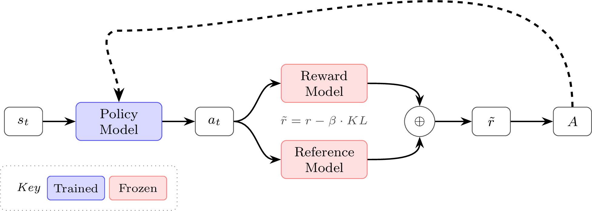
We begin with the objective:

$J(\theta) = \mathbb{E}_{\tau \sim \pi_\theta}[R(\tau)]$

This expectation can be written as a sum over all trajectories:

$J(\theta) = \sum_{\tau} P(\tau;\theta)R(\tau)$

where the probability of a trajectory is

$P(\tau;\theta) = \rho(s_0) \prod_{t=0}^{T-1} \pi_\theta(a_t|s_t) P(s_{t+1}|s_t,a_t)$

Here:

• $\rho(s_0)$ is the initial state distribution
• $\pi_\theta(a_t|s_t)$ is the policy
• $P(s_{t+1}|s_t,a_t)$ represents environment dynamics

Taking the gradient with respect to $\theta$:

$\begin{aligned} \nabla_\theta J(\theta) &= \nabla_\theta \sum_{\tau} P(\tau;\theta)R(\tau) \\ &= \sum_{\tau} R(\tau)\nabla_\theta P(\tau;\theta) \\ &= \sum_{\tau} R(\tau) P(\tau;\theta) \nabla_\theta \log P(\tau;\theta) \\ &\qquad \because \nabla_\theta P(\tau;\theta) = P(\tau;\theta)\nabla_\theta \log P(\tau;\theta) \end{aligned}$

Expanding the trajectory probability:

$P(\tau;\theta) = \rho(s_0) \prod_{t=0}^{T-1} \pi_\theta(a_t|s_t) P(s_{t+1}|s_t,a_t)$

Taking the logarithm:

$\log P(\tau;\theta) = \log \rho(s_0) + \sum_{t=0}^{T-1} \log \pi_\theta(a_t|s_t) + \sum_{t=0}^{T-1} \log P(s_{t+1}|s_t,a_t)$

Now differentiate with respect to $\theta$:

• The environment dynamics do not depend on $\theta$
• The initial state distribution also does not depend on $\theta$

Therefore,

$\nabla_\theta \log P(\tau;\theta) = \sum_{t=0}^{T-1} \nabla_\theta \log \pi_\theta(a_t|s_t)$

Substituting this back into the objective gradient gives

$\nabla_\theta J(\theta) = \mathbb{E}_{\tau \sim \pi_\theta} \left[ R(\tau) \sum_{t=0}^{T-1} \nabla_\theta \log \pi_\theta(a_t|s_t) \right]$

This is the REINFORCE gradient estimator, which forms the basis of Vanilla Policy Gradient methods.

However, using the full trajectory return $R(\tau)$ for every action can lead to very high variance. Every action is weighted using the final outcome of the entire episode, even though many rewards may not actually be caused by that specific action.

Instead, we use the future return starting from timestep $t$:

$G_t = \sum_{k=t}^{T-1} \gamma^{k-t}r_k$

The gradient now becomes

$\nabla_\theta J(\theta) = \mathbb{E} \left[ \sum_{t=0}^{T-1} \nabla_\theta \log \pi_\theta(a_t|s_t) G_t \right]$

This works because an action at timestep $t$ cannot influence rewards that occurred before timestep $t$.

Even with future returns, the gradient estimate can still have high variance. To reduce this variance, we subtract a baseline that does not depend on the sampled action:

$\mathbb{E} \left[ \nabla_\theta \log \pi_\theta(a_t|s_t) b(s_t) \right] = 0$

Therefore, the objective can be rewritten as

$\nabla_\theta J(\theta) = \mathbb{E} \left[ \sum_{t=0}^{T-1} \nabla_\theta \log \pi_\theta(a_t|s_t) \bigl( G_t - b(s_t) \bigr) \right]$

When the baseline is chosen as the value function $V^\pi(s_t)$, the quantity

$A^\pi(s_t, a_t) = G_t - V^\pi(s_t)$

is called the advantage. It measures whether an action performed better or worse than the policy's average expectation for that state.

Why use a baseline?

Without a baseline, every action is weighted directly by the raw return $G_t$. But this only tells us whether the episode outcome was good or bad overall — not whether the action itself was better or worse than expected.

This creates high variance because the return mixes together:

• The quality of the action
• The quality of the state the agent was already in

As a result, a good action taken in a bad state and a bad action taken in a good state can produce similar returns.

Subtracting a baseline centers the learning signal:

$G_t - b(s_t)$

Instead of asking:

"Was the return high?"

the policy gradient now asks:

"Was this action better or worse than expected in this state?"

Commonly used baselines include:

• Moving average reward
• Batch mean reward (used carefully in practice)
• Learned value function $V_\pi(s)$

3.

References

1. Nathan Lambert, Louis Castricato, Leandro von Werra, and Alex Havrilla. "Reinforcement Learning from Human Feedback: From Zero to Hero." rlhfbook.com, 2024.

Tags: #RL #NLP

Discussion

Add a Comment

Markdown Guide

Italics *text*

Bold **text**

Hyperlink [text](url)

Inline Code `code`

Underline __text__

Quote > text

Strikethrough ~~text~~

Comments