Multi-armed Bandits
- k-armed Bandit Problem
- Action-value Methods
- The 10-armed Testbed
- Incremental Implementation
- Nonstationary Problem
- Optimistic Initial Values
- Upper-Confidence-Bound Action Selection
- Gradient Bandit Algorithms
- Associative Search (Contextual Bandits)
- Problems
- Additional
The feature that distinguish reinforcement learning from other forms of learning is the fact that it uses training information that evaluates the actions taken rather than instructs by giving correct actions. This creates a need for exploration, to find the best action to take. Pure evaluative feedback can indicate how good the action was, but not if it is the best or worst. Purely instructive feedback, on other hand, indicates the correct action to take, independently of the action actually taken.
k-armed Bandit Problem
Its a type of problem in which we have to choose an option, or action among a set of k-options. After each action, we recieve a reward from a stationary probability distribution that depends on the action taken. The objective is to maximize the expected total reward over time.
In this problem, each of the k-actions has an expected or mean reward given that an action is taken. We call this the value of the action. Let $A_t$ denoted the action taken at time $t$, and $R_t$ the corresponding reward. Then, the value of an arbitrary action $a$, denoted $q^\star(a)$ , is the expected total reward of taking action $a$:
\[q^\star(a) = \mathbb{E}[R_t | A_t = a]\]Most of the time we don’t know the value of each actions, although we might have estimates. We denote the estimated value of action $a$ at time step $t$ as $Q_t(a)$. Also, we want $Q_t(a)$ to be as close as possible to $q^\star(a)$.
If we maintain estimates of the value of each action, then we can easily find the best action to take. The best action is the one with the highest value. We call these the greedy-action, i.e. we are exploiting the current knowledge. If we select a non-greedy action, then we are exploring, because this helps in estimating the value of non-greedy actions. Exploitation helps to maximize the rewards on one step, but exploration may help in producing better rewards over time.
Action-value Methods
Action-value methods are methods that is used for estimating the values of actions and using them to choose actions. One way to estimate the true value of the action is by averaging the rewards received:
\[\begin{align} Q_t(a) &= \frac{\text{sum of rewards when a taken prior to t}}{\text{number of times a was taken prior to t}} \\ &= \frac{\sum_{i=1}^{t-1} R_i.𝟙_{A_i = a}}{\sum_{i=1}^{t-1} 𝟙_{A_i = a}} \end{align}\]where $𝟙_{A_i = a}$ denotes the random variable that is 1 when the predicate $A_i = a$ is true, and 0 otherwise. If denominator is zero, then we define $Q_t(a)$ to be zero, or some random value. As denominator goes to infinity, $Q_t(a)$ approaches $q^\star(a)$. This method is called sample-average method because each estimate is an average of the sample of relavant rewards.
The simplest action selection rule is to select the action with the highest estimate value, that is, the greedy action as defined above. If there are multiple greedy action, then we select an action in a random manner. Mathematically,
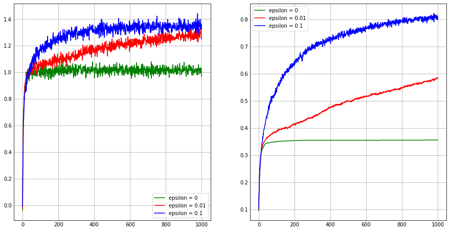
\[A_t = \underset{a}{argmax} \: Q_t(a)\]where, $argmax_a$ denotes the action $a$ for which the value $Q_t(a)$ is the largest. Greedy action selection always exploits the current knowledge to maximize immediate rewards; it does not spend time sampling the inferior actions which may have a better reward. A simple method to solve this problem is to behave greedy most the time, but there is a small probability $\epsilon$, that we randomly choose an action among all action with equal probability, independent of the action-value estimates. This method is called as $\epsilon$-greedy method. An advantage of this method is that, with increases in number of steps, every action will be sampled an infinite number of times, ensuring that all $Q_t(a)$ converges to $q^\star(a)$. Suppose an unexplored action is the optimal action, the probability of choosing this action in the beginning is just $\epsilon$, but as the number of time step increases, this action might become the optimal action. This implies that the probability of choosing optimal action converges to greater than $1-\epsilon$. These are just asymptotic guarantees, but not practically efficient.
The 10-armed Testbed
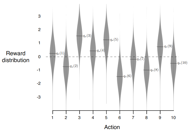
This is a set of 2000 randomly generated k-armed bandit problem with k = 10. For each problem, the action values, $q^\star(a)$, $a \in {1, \dots, k}$, are selected according to a normal(Gaussian) distribution with mean 0 and variance 1. Then, when a learning method applied to that problem selected an action $A_t$ at time step $t$, the actual reward, $R_t$, is selected from a normal distribution with mean $q^*(A_t)$ and variance 1. These distributions are shown in the figure below.
Incremental Implementation
We estimate action value as sample averages of observed rewards. But, this is computationally expensive. We also need a method to compute the average with constant memory and time complexity. For this, it is easy to devise incremental formula for updating the average with small, constant computation to process each new reward. Given $Q_n$ and the $n^{th}$ reward, the new average is:
\[\begin{align} Q_{n+1} &= \frac{1}{n}\sum_{i=1}^{n}R_i \\ &= \frac{1}{n} \left(R_n + \sum_{i=1}^{n-1} R_i\right) \\ &= \frac{1}{n} \left(R_n + (n-1)\frac{1}{n-1} \sum_{i=1}^{n-1} R_i\right) \\ &= \frac{1}{n} \left(R_n + (n-1)\times Q_n\right) \\ &= \frac{1}{n} \left(R_n + nQ_n - Q_n\right) \\ &= Q_n + \frac{1}{n} \left(R_n - Q_n\right) \end{align}\]This is of the form: $\text{Next Estimate} \leftarrow \text{Old Estimate + StepSize[Target - Old Estimate]}$.
Simple bandit algorithm - psuedo-code
The following is a psuedo-code for a bandit algorithm that uses incremental estimation. In this function bandit takes an action and returns corresponding reward.
-
Initialize, for a = 1 to k:
- $Q[a] \leftarrow 0$
- $N[a] \leftarrow 0$
-
Loop forever
- $\begin{equation} A \leftarrow \begin{cases} argmax_a\: Q(a) & \text{with probability 1-}\epsilon\\ \text{random action} & \text{with probability } \epsilon \\ \end{cases} \end{equation}$
- $R \leftarrow bandit(A)$
- $N[A] \leftarrow N[A] + 1$
- $Q[A] \leftarrow Q[A] + \frac{1}{N[A]} \left(R - Q[A]\right)$
Simple bandit algorithm - implementation
from tqdm import tqdm

import matplotlib.pyplot as plt
import numpy as np

k = 10
no_of_problem = 2000

q_star = np.random.normal(0, 1, (no_of_problem, k))
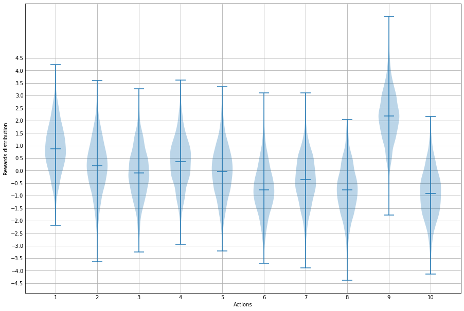
The true values $q^\star(a)$ of each of the actions is generated from a normal distribution with mean 0 and variance 1, and the actual rewards are generated from a normal distribution with mean $q^*(a)$ and variance 1.
reward_example = [np.random.normal(q_star[0, i], 1, 2000) for i in range(k)]

plt.style.use('_mpl-gallery')
plt.figure(figsize=(12,8))
plt.ylabel('Rewards distribution')
plt.xlabel('Actions')
plt.xticks(range(1,11))
plt.yticks(np.arange(-5,5,0.5))

plt.violinplot(
    reward_example,
    positions=range(1,11),
    showmeans=False,
    showextrema=True,
    showmedians = True
)
plt.show()
def bandit(action, problem):
    return np.random.normal(q_star[problem, action], 1)

def simple_bandit(k, epsilon, steps, initial_Q):
    rewards = np.zeros(steps)
    actions = np.zeros(steps)

    for i in tqdm(range(num_problems)):
        Q = np.ones(k) * initial_Q # initial Q
        N = np.zeros(k)  # initalize number of rewards given
        for t in range(steps):
            best_action = np.argmax(q_star[i])
            if np.random.rand() < epsilon:
                # exploration
                a = np.random.randint(k)
            else:
                # exploitation - choose one random action in case of tie
                a = np.random.choice(
                    np.where(Q == Q.max())[0]
                )

            reward = bandit(a, i)

            N[a] += 1
            Q[a] = Q[a] + (reward - Q[a]) / N[a]

            rewards[t] += reward

            if a == best_action:
                actions[t] += 1

    return np.divide(rewards,num_problems), np.divide(actions,num_problems)

ep_0, ac_0 = simple_bandit(k, no_of_problem, epsilon=0, steps=1000, initial_Q=0)
ep_01, ac_01 = simple_bandit(k, no_of_problem,  epsilon=0.01, steps=1000, initial_Q=0)
ep_1, ac_1 = simple_bandit(k, no_of_problem,  epsilon=0.1, steps=1000, initial_Q=0)
plt.figure(figsize=(12,6))
plt.subplot(1,2,1)
plt.plot(ep_0, 'g', label='epsilon = 0')
plt.plot(ep_01, 'r', label='epsilon = 0.01')
plt.plot(ep_1, 'b', label='epsilon = 0.1')
plt.legend()
plt.subplot(1,2,2)
plt.yticks(np.arange(0,1,0.1))
plt.plot(ac_0, 'g', label='epsilon = 0')
plt.plot(ac_01, 'r', label='epsilon = 0.01')
plt.plot(ac_1, 'b', label='epsilon = 0.1')
plt.legend()
plt.show()
Nonstationary Problem
These are the problems in which the distribution changes over time. For example, the probability of coin toss outcome changes due to wear and tear of the coin. In such cases, its better to give more weight to the recent rewards rather than to the long-past rewards. One way to this is to use a constant step size. That is, the incremental rule is modified to: $Q_{t+1} = Q_t + \alpha \left( R_t - Q_t \right)$, where $\alpha \in (0,1]$. This results in $Q_{t+1}$ being a weighted average of past rewards and the initial estimate $Q_0$.
\[\begin{align} Q_{t+1} &= Q_t + \alpha \left( R_t - Q_t \right) \\ &= \alpha R_t + (1-\alpha) Q_t \\ &= \alpha R_t + (1-\alpha)[\alpha R_{t-1} + (1-\alpha)Q_{t-1}] \\ &= \alpha R_t + (1-\alpha)\alpha R_{t-1} + (1-\alpha)^2Q_{t-1} \\ &\text{...........................................................} \\ &\text{...........................................................} \\ &= (1-\alpha)^tQ_1 + \sum_{i=1}^t \alpha(1-\alpha)^{t-i} R_i \\ \end{align}\]This is actually a weighted average because the sum of the weights is $(1-\alpha)^t + \sum_{i=1}^t \alpha(1-\alpha)^{t-i} = 1$. Here, the quantity $1-\alpha$ is less than zero, so the weight given to $R_i$ starts to decrease as the number of intervening rewards increases. The weight decays exponentially according to the exponent on $1-\alpha$
Sometimes its convenient to vary the step-size parameter from step-to-step. Let $\alpha_n(a)$ denoted the step-size parameter at the $n^th$ selection of action $a$. We know that $\alpha_n(a) = \frac{1}{n}$ is guaranteed to converge to the true action values by the law of large numbers. But convergence is not guaranteed for all choices of the sequence ${\alpha_n(a)}$. In stochastic approximation theory there are two conditions that must be satisfied to assure the convergence with probability of 1:
- $\sum_{n=1}^{\infty} \alpha_n(a) = \infty$
- $\sum_{n=1}^{\infty} \alpha^2_n(a) < \infty$
The first condition is needed to ensure that the steps are large enough to eventually overcome any initial conditions or random fluctuations. The second guarantees that eventually the steps become small enough to assure the convergence.
We can see that for $\alpha_n(a) = \frac{1}{n}$, both conditions are satisfied. But for constant step-size parameter, $\alpha_n(a) = \alpha$, only the first condition is satisfied. This indicates that estimates never completely converge but continue to vary in response to most recently received rewards.
Optimistic Initial Values
Most of the previous methods depends on the initial vallue estimate $Q_1(a)$. That is these methods are biased by their initial value estimate. For sampling average method, the bias will disappear once all the actions are selected at least once. But for methods with constant step-size parameter, the bias is permanent, though it decrease over time. The problem with this is that it becomes a parameter which the user must tune, but sometimes when the user wants to apply prior knowledge this comes handy.
Suppose we use an initial estimate of +5 for all action. This actually encourage the action-value method to explore more. Whichever action is selected in the beginning, the reward is less than starting estimate. That is $R - Q(a)$ will be negative which causes Q(a) to decrease for a while and this in turn causes more exploration in the beginning. This in turns causes the action-value method to explore more. But this isn’t suitable for non-stationary problems because the exploration is temporary.
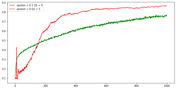
Figure above shows the effect of optimistic initial estimates on the 10-armed testbed. Both method use a constant step-size parameter, $\alpha = 0.1$.
Upper-Confidence-Bound Action Selection
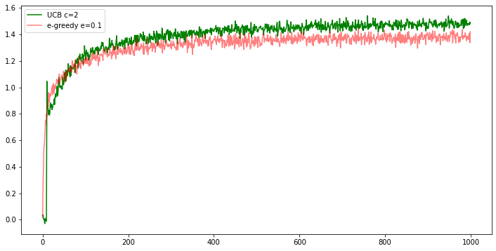
We know $\epsilon$-greedy action chooses action greedily even though it sometimes forces the non-greedy actions to be tried. In this case, it would be better if we can select non-greedy actions, but those with the potential of being optimal, taking into account both how close their estimates are to being maximal and the uncertainities in those estimates. One way to perform this is by selecting actions according to:
\[\begin{align} A_t = \underset{a}{argmax}\left[Q_t(a) + c\sqrt{\frac{\ln(t)}{N_t(a)}}\right] \\ \end{align}\]where $c$ is a constant such that $c > 0$ and $N_t(a)$ is the number of times action $a$ was selected. If $N_t(a) = 0$, then a is considered to be a maximizing action.
The idea of UCB action selection is that the square-root term is a measure of the uncertainty or variance in the estimate of the action-value function. Each time an action $a$ is selected the uncertainty is reduced: $N_t(a)$ increases, and this causes the term $\frac{\ln(t)}{N_t(a)}$ to approach zero. Thus exploration reduces as time-step increases. On the other hand, each time an other action is selected, $t$ increases but not $N_t(a)$. This causes the term $\frac{\ln(t)}{N_t(a)}$ to increase. This increases the uncertainty and thus the exploration. Logarithm is used, so that this increase gets smaller over time, but actions with lower value estimates, or that have been selected frequenly, will be selected with decreasing frequency.
Implementation
k = 10
no_of_problem = 2000

def bandit_UCB(action, problem):
    result = np.random.normal(q_star[problem, action], 1)
    return result

def simple_bandit_UCB(k, num_problems, epsilon, c, steps, initial_Q):
    rewards = np.zeros(steps)
    actions = np.zeros(steps)

    for i in tqdm(range(num_problems)):
        Q = np.ones(k) * initial_Q # initial Q
        N = np.zeros(k)  # initalize number of rewards given

        for t in range(steps):
            best_action = np.argmax(q_star[i])
            if np.random.rand() < epsilon:
                # exploration
                a = np.random.randint(k)
            else:
                # exploitation - choose one random action in case of tie
                if N.all():
                    Q_ = Q+c*(np.sqrt(np.log(t)/N))
                    a = np.random.choice(
                        np.where(Q_ == Q_.max())[0]
                    )
                else:
                    a = np.random.choice(
                        np.where(N == 0)[0]
                    )


            reward = bandit_UCB(a, i)

            N[a] += 1
            Q[a] = Q[a] + (reward - Q[a]) / N[a]

            rewards[t] += reward

            if a == best_action:
                actions[t] += 1

    return np.divide(rewards,num_problems), np.divide(actions,num_problems)

in_ep, in_ac = simple_bandit_UCB(
    k, no_of_problem, epsilon=0 , c=2, steps=1000, initial_Q=0
    )
co_ep, co_ac = simple_bandit(
    k, no_of_problem, epsilon=0.1, steps=1000, initial_Q=0
    )

plt.figure(figsize=(12,6))
plt.plot(in_ep, 'g', label='UCB c=2')
plt.plot(co_ep, 'r', label='e-greedy e=0.1', alpha=0.5)
plt.legend()
plt.savefig('foo.png', bbox_inches='tight')
Gradient Bandit Algorithms
In this method, agent learns a numerical preference for each action $a$, which is denoted as $H_t(a)$. The larger the preference is for an action, the more likely the agent will choose that action. But this preference has no interpretation in terms of reward. The relative preference of one action to another is important. This preferences are determined according to a softmax distribution:
\[\begin{align} Pr\{A_t = a\} = \frac{e^{H_t(a)}}{\sum_{j=1}^k e^{H_t(j)}} = \pi_t(a) \\ \end{align}\]Here, $\pi_t(a)$ is the probability of choosing action $a$ at time $t$. Initially all action preferences are the same so that all actions are equally likely to be chosen.
On each step, after selecting an action $A_t$ and receiving a reward $R_t$, the agent updates its preference for each action as:
\[\begin{equation} H_{t+1}(A_t) = H_t(A_t) + \alpha \left(R_t - \bar{R}_t\right)(1- \pi_t(A_t)) \\ H_{t+1}(a) = H_t(a) - \alpha \left(R_t - \bar{R}_t\right)(\pi_t(a)) \quad \forall a \neq A_t \\ \end{equation}\]where $\bar{R}_t \in \mathbb{R}$ is the average reward over the last $t$ steps. $\bar{R}_t$ serves as a baseline with which the reward is compared. If reward is higher than the baseline, then the probability of taking action $A_t$ increases. If reward is lower than the baseline, then the probability of taking action $A_t$ decreases.
Implementation
Here, the true reward is selected according to a normal distribution with mean of +4 and unit variance.
k = 10
no_of_problem = 200

q_star = np.random.normal(4, 1, (no_of_problem, k))

def calculate_softmax(H):
    e_H = np.exp(H - np.max(H))
    return (e_H / e_H.sum())

def bandit(action, problem):
    return np.random.normal(q_star[problem, action], 1)

def gradient_bandit(k, num_problems, alpha, steps, baseline = False):
    rewards = np.zeros(steps)
    actions = np.zeros(steps)

    for i in tqdm(range(num_problems)):

        H = np.zeros(k)
        RT = 0
        best_action = np.argmax(q_star[i])
        step_reward = []
        for t in range(steps):
            softmax = calculate_softmax(H)
            a = np.random.choice(
                k, 1, p = softmax
            )[0]
            reward = bandit(a, i)

            H[a] = H[a] + alpha * (
                reward - RT
            )*(1 - softmax[a])

            for j in [k for k in range(10) if k != a]:
                H[j] = H[j] - alpha * (
                    reward - RT
                )*(softmax[j])

            rewards[t] += reward
            step_reward.append(reward)

            if a == best_action:
                actions[t] += 1

            if baseline:
                RT = np.average(np.array(step_reward))


    return np.divide(rewards,num_problems), np.divide(actions,num_problems)

r01, a01 = gradient_bandit(k, no_of_problem, alpha=0.1, steps=1000)
r04, a04 = gradient_bandit(k, no_of_problem, alpha=0.4, steps=1000)
r01B, a01B = gradient_bandit(k, no_of_problem, alpha=0.1, steps=1000, baseline = True)
r04B, a04B = gradient_bandit(k, no_of_problem, alpha=0.4, steps=1000, baseline = True)

plt.figure(figsize=(12,6))
plt.yticks(np.arange(0,1,0.1))
plt.plot(a01B, 'g', label='alpha = 0.1 Baseline')
plt.plot(a04B, 'g', label='alpha = 0.4 Baseline', alpha = 0.6)
plt.plot(a01, 'r', label='alpha = 0.1')
plt.plot(a04, 'r', label='alpha = 0.4', alpha = 0.6)
plt.legend()
plt.savefig('foo.png', bbox_inches='tight')
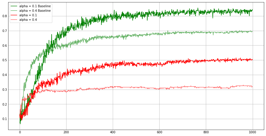
Note that when performance significanly degraded when omitted the baseline($R_t = 0$).
Associative Search (Contextual Bandits)
In nonassociative tasks, there is no need to associate different actions with different situations. Here, the agent tries to find a single best action when task is stationary or tries to track the best action when task is non-stationary. However in general reinforcement learning task there is a more than one situation, and the goal is to learn a policy: a mapping from situations to actions that are best for the situation.
Associative search tasks are those which involves both trial-and-error learning to search for best action, and association of these actions with the situations in which they are best.
Problems
-
In $\epsilon$-greedy action selection, for the case of two actions and $\epsilon$ = 0.5, what is the probability that the greedy action is selected?
\(\begin{align*} P(\text{greedy action}) &= P(\text{greedy action by greedy selection}) + P(\text{greedy action by random selection}) \\ &= P(\text{greedy selection}) * P(\text{greedy action | greedy selection}) \\ &\quad\quad + P(\text{random selection}) * P(\text{greedy action | random selection}) \\ &= \epsilon*1 + (1-\epsilon) * 0.5 \\ &= 0.5*1 + 0.5*0.5 \\ &= 0.75 \end{align*}\)
-
Consider a k-armed bandit problem with k = 4 actions, denoted 1, 2, 3, and 4. Consider applying to this problem a bandit algorithm using ε-greedy action selection, sample-average action-value estimates, and initial estimates of $Q_1(a) = 0$, for all $a$. Suppose the initial sequence of actions and rewards is $A_1 = 1, R_1 = -1, A_2 = 2, R_2 = 1, A_3 = 2, R_3 = -2, A_4 = 2, R_4 = 2, A_5 = 3, R_5 = 0$. On some of these time steps the ε case may have occurred, causing an action to be selected at random. On which time steps did this definitely occur? On which time steps could this possibly have occurred?
$Q^0 = \begin{bmatrix}0 & 0 & 0 & 0\end{bmatrix}$
$A^1 = 1 \implies Q^1 = \begin{bmatrix}-1 & 0 & 0 & 0\end{bmatrix}$
$A^2 = 2 \implies Q^2 = \begin{bmatrix}-1 & 1 & 0 & 0\end{bmatrix}$
$A^3 = 2 \implies Q^3 = \begin{bmatrix}-1 & \frac{-1}{2} & 0 & 0\end{bmatrix}$
$A^4 = 2 \implies Q^4 = \begin{bmatrix}-1 & \frac{1}{3} & 0 & 0\end{bmatrix}$
$A^5 = 3 \implies Q^5 = \begin{bmatrix}-1 & \frac{1}{3} & 0 & 0\end{bmatrix}$Choosing $A_1 = 1$ can be greedy or random, $A_2 = 2$ can also be greedy or random, $A_3 = 2$ is greedy but can also be due to random selection, $A_4 = 2$ can be greedy or random, $A_5 = 3$ is definitely random.
-
In the comparision shown in figure, which method will perform best in the long run in terms of cumulative reward and probability of selecting the best action? How much better will it be? Express your answer quantitatively.
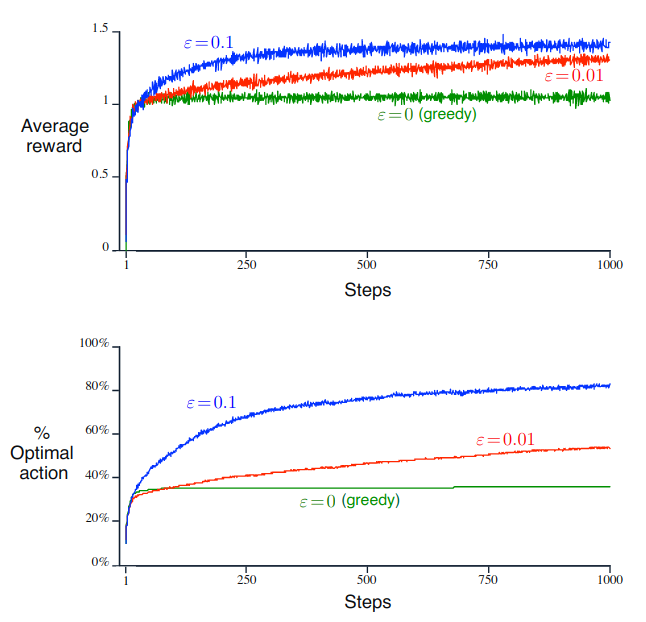
Let probability for random selection be $\epsilon$ and probability for greedy selection be 1 - $\epsilon$. Let $a^*$ denote the optimal action and $n$ denotes the number of choice. Then,
$p(A = a^\star) = \epsilon\times\frac{1}{n} + (1-\epsilon) \times 1$
For this problem, n = 10 and probability of choosing greedy solution while greedy approach is 1 and while random approach is $\frac{1}{10}$.$p(A = a^*) = \epsilon*0.1 + (1-\epsilon)$
\(\begin{equation} p(A = a^*) = \begin{cases} 0.91 & \text{if } \epsilon = 0.1 \\ 0.991 & \text{if } \epsilon = 0.01 \\ \end{cases} \end{equation}\)Let $r^\star$ denote the optimal reward. Then,
$E[R = r^\star] = p(A = a^\star) \times r^\star + (1-p(A = a^\star)) \times 0$
$E[R = r^\star] = (\epsilon*0.1 + (1-\epsilon)) \times r^\star$
\(\begin{equation} E[R = r^\star] = \begin{cases} 0.91*r^\star & \text{if } \epsilon = 0.1 \\ 0.991*r^\star & \text{if } \epsilon = 0.01 \\ \end{cases} \end{equation}\)Therefore, this method performs best when $\epsilon$ = 0.01, although it looks $\epsilon$ = 0.1 is better.
-
If the step-size parameters, $\alpha_n$, are not constant, then the estimate $Q_n$ is a weighted average of previously received rewards with a weighting different from that given by (2.6). What is the weighting on each prior reward for the general case, analogous to (2.6), in terms of the sequence of step-size parameters?
\(\begin{align} Q_{n+1} &= Q_n + \alpha_n[R_n - Q_n] \\ &= \alpha_nR_n + (1-\alpha_n)Q_n \\ &= \alpha_nR_n + (1-\alpha_n)(\alpha_{n-1}R_{n-1} + (1-\alpha_{n-1})Q_{n-1}) \\ &................................\\ &................................ \\ &= Q_1\prod_{i=1}^{n}(1-\alpha_i) + \sum_{i=1}^{n}\alpha_i R_{i}\prod_{j=i+1}^{n}(1-\alpha_j) \\ \end{align}\) -
Design and conduct an experiment to demonstrate the difficulties that sample-average methods have for nonstationary problems. Use a modified version of the 10-armed testbed in which all the $q^\star(a)$ start out equal and then take independent random walks (say by adding a normally distributed increment with mean zero and standard deviation 0.01 to all the $q^\star(a)$ on each step). Prepare plots like Figure 2.2 for an action-value method using sample averages, incrementally computed, and another action-value method using a constant step-size parameter, $\alpha=0.1$. Use $\epsilon=0.1$ and longer runs, say of 10,000 steps.
 k = 10
 no_of_problem = 200
 q_star = np.random.normal(0, 0, (no_of_problem, k))

 def bandit_NS(action, problem):
 result = np.random.normal(q_star[problem, action], 1)
 q_star[problem] += np.random.normal(0, 0.01, q_star[problem].shape)
 return result

 def simple_bandit_NS(k, num_problems, alpha, epsilon, steps, initial_Q):
     rewards = np.zeros(steps)
     actions = np.zeros(steps)

     q_star.fill(0)

     for i in tqdm(range(num_problems)):
         Q = np.ones(k) * initial_Q # initial Q
         N = np.zeros(k)  # initalize number of rewards given

         for t in range(steps):
             best_action = np.argmax(q_star[i])
             if np.random.rand() < epsilon:
                 # exploration
                 a = np.random.randint(k)
             else:
                 # exploitation - choose one random action in case of tie
                 a = np.random.choice(
                     np.where(Q == Q.max())[0]
                 )

             reward = bandit_NS(a, i)

             N[a] += 1
             if alpha > 0:
                 Q[a] = Q[a] + (reward - Q[a])*alpha
             else:
                 Q[a] = Q[a] + (reward - Q[a]) / N[a]

             rewards[t] += reward

             if a == best_action:
                 actions[t] += 1

     return np.divide(rewards,num_problems), np.divide(actions,num_problems)

 in_ep, in_ac = simple_bandit_NS(
     k, no_of_problem, alpha=0, epsilon=0.1, steps=10000, initial_Q=0
     )
 co_ep, co_ac = simple_bandit_NS(
     k, no_of_problem, alpha=0.1, epsilon=0.1, steps=10000, initial_Q=0
     )

 plt.figure(figsize=(20,6))
 plt.subplot(1,2,1)
 plt.plot(in_ep, 'g', label='epsilon = 0.1 alpha=0')
 plt.plot(co_ep, 'r', label='epsilon = 0.1 alpha=0.1', alpha=0.5)
 plt.legend()
 plt.subplot(1,2,2)
 plt.yticks(np.arange(0,1,0.1))
 plt.plot(in_ac, 'g', label='epsilon = 0.1 alpha=0')
 plt.plot(co_ac, 'r', label='epsilon = 0.1 alpha=0.1', alpha=0.5)
 plt.legend()
 plt.savefig('foo.png', bbox_inches='tight')
-
Mysterious Spikes The results shown in Figure 2.3 should be quite reliable because they are averages over 2000 individual, randomly chosen 10-armed bandit tasks. Why, then, are there oscillations and spikes in the early part of the curve for the optimistic method? In other words, what might make this method perform particularly better or worse, on average, on particular early steps?
The optimistic method in beginning explores all the actions. This is because value estimates are greater than the true value. Eventhough it chooses the optimal action it forgets that action and explores other actions because the algorithm reduce the Q values in the beginning.
-
Unbiased Constant-Step-Size Trick In most of this chapter we have used sample averages to estimate action values because sample averages do not produce the initial bias that constant step sizes do (see the analysis leading to(2.6)). However, sample averages are not a completely satisfactory solution because they may perform poorly on nonstationary problems. Is it possible to avoid the bias of constant step sizes while retaining their advantages on nonstationary problems? One way is to use a step size of
$\beta_n \dot{=} \alpha / \bar{o}_n$
to process the $n^{th}$ reward for a particular action, where $\alpha > 0$ is a conventional constant step size, and $\bar{o}_n$ is a trace of one that starts at 0:
$\overline{o}_n \dot{=} \overline{o}_{n-1} + \alpha(1-\overline{o}_{n-1})$, for $ n \geq 0$, with $\overline{o}_0 \dot{=} 0$
Carry out an analysis like that in (2.6) o show that $Q_n$ is an exponential recency-weighted average without initial bias.If we look into problem 4, we can see that $Q_{n+1} = Q_1\prod_{i=1}^{n}(1-\alpha_i) + \sum_{i=1}^{n}\alpha_i R_{i}\prod_{j=i+1}^{n}(1-\alpha_j)$.
Here, for this case equation becomes $Q_{n+1} = Q_1\prod_{i=1}^{n}(1-\beta_i) + \sum_{i=1}^{n}\beta_i R_{i}\prod_{j=i+1}^{n}(1-\beta_j)$.When i = 1, $\bar{o}_1 = \bar{o}_0 + \alpha(1 - \bar{o}_0)$. Given that $\bar{o}_0 = 0 \implies \bar{o}_1 = \alpha$. Therefore, $\beta_1 = 1$
This implies that the equation is independent of initial estimate, because the term $Q_1\prod_{i=1}^{n}(1-\beta_i)$ becomes 0, after $i=1$.
-
UCB Spikes In Figure 2.4 the UCB algorithm shows a distinct spike in performance on the 11th step. Why is this? Note that for your answer to be fully satisfactory it must explain both why the reward increases on the 11th step and why it decreases on the subsequent steps. Hint: if c = 1, then the spike is less prominent.
In the first 10 steps, all actions are explored since $N_t(a) = 0$. But in the 11th step, the action chooses the best action. Note that the uncertainty term won’t affect the action since $t$ and $N_t(a)$ is same for all actions. Now upper confidence bound for this action decreases ($N_t(a)$ increases) and for the other actions increases. $c$ being a large value, amplifies the certainity thus causing the agent to choose an another action, which is less valuable. And this reason causes the reward to decrease in the following steps. As time-step increases, this effect decreases.
-
Show that in the case of two actions, the soft-max distribution is the sameas that given by the logistic, or sigmoid, function often used in statistics and artificial neural networks.
$Pr \{ A_t = a\} \dot{=} \frac{\Large{e^{H_t(a)}}}{\Large{\sum_{i=1}^{K}e^{H_t(i)}}}$
For two actions a and b, the distribution becomes:
\[\begin{align} Pr\{A_t = a\} &= \frac{e^{H_t(a)}}{e^{H_t(a)} + e^{H_t(b)}} \\ &= \frac{1}{1 + e^{H_t(b) - H_t(a)}} \end{align}\]We know that sigmoid function is: \(f(x) = \frac{1}{1 + e^{-x}}\)
Here, this distribution is same as sigmoid distribution, when $x = -(H_t(b) - H_t(a))$.
-
Suppose you face a 2-armed bandit task whose true action values change randomly from time step to time step. Specifically, suppose that, for any time step, the true values of actions 1 and 2 are respectively 0.1 and 0.2 with probability 0.5 (case A), and 0.9 and 0.8 with probability 0.5 (case B). If you are not able to tell which case you face at any step, what is the best expectation of success you can achieve and how should you behave to achieve it? Now suppose that on each step you are told whether you are facing case A or case B (although you still don’t know the true action values). This is an associative search task. What is the best expectation of success you can achieve in this task, and how should you behave to achieve it?
1) If we don’t know what state we are in, then the best we could do in this situation is to choose the same action for all steps. Thus,
$\mathbb{E}[R | 1] = 0.1\times 0.5 + 0.9\times 0.5 = 0.5$
$\mathbb{E}[R | 2] = 0.2\times 0.5 + 0.8\times 0.5 = 0.5$
The best expected reward is 0.5.2) When we know in what state we are in, we can choose action 2 from case A and action 1 from case 2. In this case the best expectation we get is:
$\mathbb{E}[R] = 0.2\times 0.5 + 0.9\times 0.5 = 0.55$
The best expected reward is 0.55.
Additional
The Bandit Gradient Algorithm as Stochastic Gradient Ascent
We need to increment action preference $H_t(a)$ proportional to the increment’s effect on performance. i.e.
\[H_{t+1}(a) = H_t(a) + \alpha \frac{\partial \mathbb{E}[R_t]}{\partial H_t(a)}\]where $\mathbb{E}[R_t] = \sum_x\pi_t(x)q_\star(x)$ is the expected reward.
So,
\[\begin{align} \frac{\partial \mathbb{E}[R_t]}{\partial H_t(a)} &= \frac{\partial}{\partial H_t(a)}\left[\sum_x\pi_t(x)q_\star(x)\right] \\ &= \sum_x q_\star(x) \frac{\partial \pi_t(x)}{\partial H_t(a)} \\ &= \sum_x (q_\star(x) - B_t) \frac{\partial \pi_t(x)}{\partial H_t(a)} \\ \end{align}\]where $B_t$ is the baseline, that can be any scalar which doesn’t depends on $x$. Here we can add $B_t$ without changing equality because gradient sums to zero over all actions. For some actions it may go up and down for the others, but sum of changes will be zero because the sum of probability is always 1.
\[\begin{align} \frac{\partial \mathbb{E}[R_t]}{\partial H_t(a)} &= \sum_x \frac{\pi_t(x)}{\pi_t(x)} (q_\star(x) - B_t) \frac{\partial \pi_t(x)}{\partial H_t(a)} \\ \end{align}\]Equation is now of the form of expectation, summing over all values x of random variable $A_t$.
\[\begin{align} &= \mathbb{E}[\frac{1}{\pi_t(x)}(q_\star(x) - B_t)\frac{\partial \pi_t(x)}{\partial H_t(a)}] \\ &= \mathbb{E}[\frac{1}{\pi_t(x)}(R_t - bar{R}_t)\frac{\partial \pi_t(x)}{\partial H_t(a)}] \\ \end{align}\]Here, baseline $B_t = \bar{R}_t$ and $q_\star(A_t) = R_t$, which is permitted because $\mathbb{E}[R_t|A_t] = q_\star(A_t)$. Now before move on to solving this we will simplify $\frac{\partial \pi_t(x)}{\partial H_t(a)}$.
\[\begin{align} \frac{\partial \pi_t(x)}{\partial H_t(x)} &= \frac{\partial}{\partial H_t(a)} \left[ \frac{e^{H_t(a)}}{\sum_{y=1}^k e^{H_t(y)}}\right] \\ &= \frac{\frac{\partial e^{H_t(x)}}{\partial H_t(a)}\sum_{y=1}^{k} e^{H_t(y)} - e^{H_t(x)}\frac{\partial \sum_{y=1}^{k} e^{H_t(y)}}{\partial H_t(a)} }{(\sum_{y=1}^k e^{H_t(y)})^2} \text{(by quotient rule)} \\ &= \frac{𝟙_{a=x}e^{H_t(x)} \sum_{y=1}{k} e^{H_t(y)} - e^{H_t(x)}e^{H_t(a)}}{ \left( \sum_{y=1}^{k} e^{H_t(y)}\right)^2 } \\ &= \frac{𝟙_{a=x}e^{H_t(x)}}{\sum_{y=1}^{k} e^{H_t(y)}} - \frac{e^{H_t(x)} e^{H_t(a)}}{\left(\sum_{y=1}^{k} e^{H_t(y)}\right)^2} \\ &= 𝟙_{a=x}\pi_t(x) - \pi_t(x)\pi_t(a) \\ &= \pi_t(x)(𝟙_{a=x} - \pi_t(a)) \end{align}\]where, 𝟙 is 1 when predicate is true, 0 otherwise.
So now solving the rest,
\[\begin{align} &= \mathbb{E}[\frac{1}{\pi_t(x)}(R_t - bar{R}_t)\frac{\partial \pi_t(x)}{\partial H_t(a)}] \\ &= \mathbb{E}[\frac{1}{\pi_t(x)}(R_t - bar{R}_t)\pi_t(x)(𝟙_{a=x} - \pi_t(a))] \\ &= \mathbb{E}[(R_t - bar{R}_t)(𝟙_{a=x} - \pi_t(a))] \end{align}\]Substituiting a sample of the expectation above yields:
\[\begin{align} H_{t+1}(a) = H_t(a) + \alpha(R_t - \bar{R}_t)(𝟙_{a=x} - \pi_t(a))\\ \end{align}\]