• Types of feedback
  • Sequential feedback
  • Valuative feedback
  • Sampled feedback
• Function approximation for RL
  • High dimensional state and action spaces
  • Continuous state and action spaces
  • Advantages of function approximation
    • The cart-pole problem
    • Using function approximation
• NFQ: Neural fitted Q
  • Selecting a value function to approximate
  • Selecting a neural network architecture
  • Selecting what to optimize
  • Selecting the targets for policy evaluation
  • Selecting an exploration strategy
  • Selecting a loss function
  • Selecting an optimization method

Types of feedback

In deep reinforcement learning(DRL), we build agents which are capable of learning from feedback that’s simultaneously evaluative, sequential, and sampled.

Sequential feedback

DRL agents have to deal with sequential feedback. One of the problem due to this is that the agent can recieve delayed information. For instance, in a chess game we make a few wrong moves early on, but the consequence of these moves are not felt until much later in the game.

Delayed feedback makes it tricky to interpret the source of the feedback. Sequential feedback gives rise to temporal credit assignment problem, which is the challenge of determining which states, action, or state-action pairs are responsible for a reward. It becomes challenging to assign credit for rewards when there is a temporal component to a problem and the actions have delayed consequences.

The opposite of delayed feedback is immediate feedback. In other words, the opposite of sequential feedback is one-shot feedback. In problems that deal with one-shot feedback, such as supervised learning or multi-armed bandit, decisions don’t have long term consequences. For example, In a classification problem, classifying an image, whether correctly or not, has no bearing on future performance. But in DRL, this sequential dependency exists.

Valuative feedback

DRL, tabular reinforcement learning, and bandits all deal with evaluative feedback. The crux of evaluative feedback is that the goodness of feedback is only relative, because the environment is uncertain. We don’t know the actual dynamics of the environment.

As a result, we will have to explore the environment. The problem with exploration is that we miss capitalizing on our current knowledge and, therefore, likely accumulate regret. Out of all this, the exploration-exploitation trade-off arises. It’s constant by-product of uncertainity. While not having access to the model of environment, we must explore to gather new information or improve on out current information.

The oppposite of evaluative feedback is supervised feedback. In classification problem, the model receives supervision.

When under evaluative feedback, agents must balance exploration versus exploitation requirements. If the feedback is both evaluative and sequential at the same time, the challenge is more significant. Algorithms must simultaneously balance immediate- and long-term rewards and the gathering and utilization of information. Both tabular and DRL agents learn from feedback that’s simultaneously evaluative and sequential.

Sampled feedback

What differentiates DRL from tabular RL is the complexity of the problems. In DRL, agents are unlikely to sample all possible feedback exhaustively. Agents need to generalize using the gathered feedback and come up with intelligent strategies based on that generalization. Generalizing helps to narrow down the search space and focus on the most important information.

Supervised learning deals with sampled feedback. Indeed, the core challenge in supervised learning is to learn from sampled feedback: to be able to generalize to new samples, which is something neither multi-armed bandits nor tabular RL can do.

The opposite of sampled feedback is exhaustive feedback. That means the agent has access to all possible samples. To gather exhaustive feedback is a reason for optimal convergence guarantee in tabular RL.

Function approximation for RL

High dimensional state and action spaces

The main drawback of tabular reinforcement learning is that usage of tables to represent value function is not practical in complex problems. Environments can have high dimensional state spaces, meaning that the number of variables that compromises a single state is vast. For example, Atari games are high dimensional because of 210x160x3 pixels.

Continuous state and action spaces

Environments can additionally have continuous variables, meaning that a variable can take on an infinite number of values. Even if the variables aren’t continuous and, therefore, not infinitely large, they can still take on a large number of values to make it impractical for learning withoout function approximation.

Sometimes even low-dimension state spaces can be infinitely large state spaces. For example, imagine a robot in an environment represented using x,y, and z coordinates. Suppose the variables are provided in a continuous form, that is, that variable can be of infinitesimal precision. It can be like 1.7, or 1.7553, or 1.7553456, and so on. So making table that takes all values into the account is not practical. But instead, we can discretize the state space using function approximation.

Advantages of function approximation

The cart-pole problem

• The cart-pole problem is a classic in reinforcement. The state space is low dimensional but continuous.
  
  

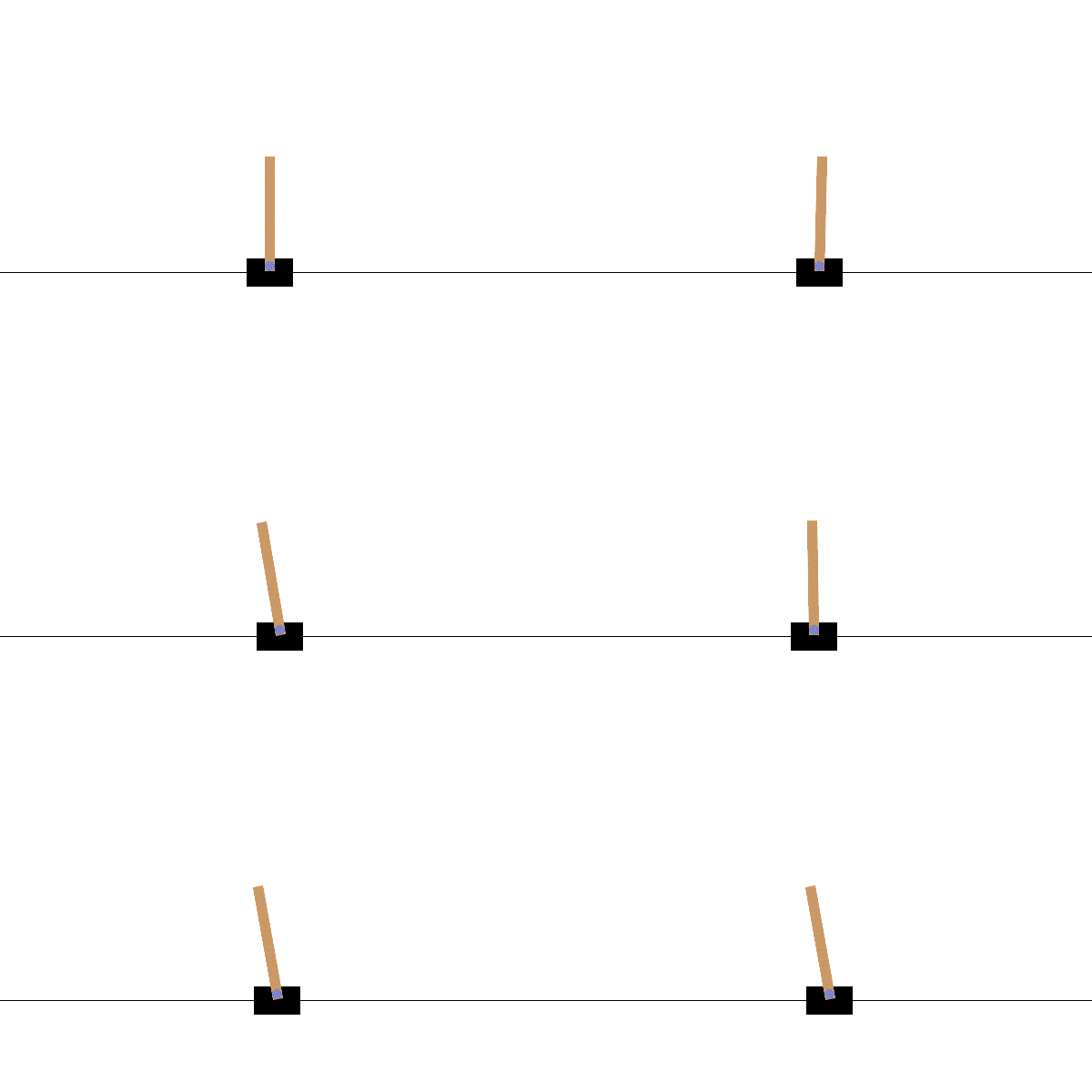
Its space comprises of four variables:

• Cart position (x-axis) with a range of [-2.4, 2.4]
• cart velocity (x-axis) with a range of [-inf, inf]
• pole angle with a range of ~[-40, 40] degrees
• pole velocity at tip with a range of [-inf, inf]

There are two available actions in every state:

• Action 0: applies a force of -1 to the cart(push left)
• Action 1: applies a force of 1 to the cart(push right)

We reach terminal state if:

• pole angle is more than 12 degree away from vertical position
• cart center is more than 2.4 units away from center of the track
• episode count reaches 500 time steps

The reward function is:

• 1 for every time step

Using function approximation

In the cart-pole environment, we want to use generalization because it’s a more efficient use of experience. With function approximation, agents learn and exploit patterns with less data.

A state-value function with and without function approximation

• Imagine a state-value function, V = [-2.5, -1.1, 0.7, 3.2, 7.6]
• Without function approximation, each value is independent.
  
  
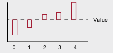
• With function approximation, the underlying relationship of the states can be learned and exploited.
  
  
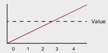
• Without function approximation, the update only changes one state.
  
  
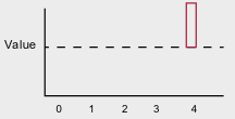
• With function approximation, the update change multiple states.
  
  
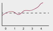
• With a non-linear function approximator, such as neural network, more complex relationship can be discovered.

While the inability of value iteration and Q-learning to solve problems with sampled feedback make them impractical, the lack of generalization makes them inefficient.

Our motivation for using function approximation isn’t only to solve the problems that aren’t solvable otherwise, but also to solve problems more efficiently.

NFQ: Neural fitted Q

The algorithm called neural fitted Q (NFQ) iteration is probably one of first algorithms to successfully use neural networks as a function approximation to solve reinforcement learning problems.

Selecting a value function to approximate

Using neural networks to approximate value functions can be done in many different ways. There are different value function which we could approximate. For example, the state value function $v(s)$, the action-value function $q(s,a)$, and the action-advantage function $a(s,a)$.

Selecting a neural network architecture

We will have to learn the approximate action-value function $Q(s, a; \theta)$, where $\theta$ is the weights of the neural network, $s$ is the state, and $a$ is the action.

A straightforward neural network architecture is to input the state, and the action to be evaluate. The output would then be one node representing the Q-value for that state-action pair.

This approach would work fine for cart-pole environment. But, a more efficient architecture consists of only inputting the state to neural network and outputting the Q-values for all the actions in that state. This is advantageous when using exploration strategies such as epsilon-greedy or softmax, because having to do only one pass forward to get the values of all actions for any state yields a high performance implementation, especially on environments with a large number of actions.

Selecting what to optimize

An ideal objective in value based DRL would be to minimize the loss with respect to the optimal action value function $q^\star$.

\[L_i(\theta) = \mathbb{E}_{s,a} \left[ \left( q^\star(s,a) - Q(s,a; \theta) \right)^2 \right]\]

But the problem with this is that we don’t have the optimal action-value function $q^\star(s, a)$, and to the top off that, we cannot even sample these optimal Q-values because we don’t have the optimal policy either. Fortunately, we can use the same principles learned in generalized policy iteration in which we alternate between policy-evaluation and policy-improvement processes to find good policies. But because of using a non-linear function approximation, convergence is not guaranteed.

Selecting the targets for policy evaluation

There are multiple ways we can evaluate a policy. More specifically, there are different targets we can use to estimate action-value function of a policy $\pi$. Ssome of them includes Monte Carlo target, temporal-difference, n-step target and lambda target.

We will use TD methods for now. The off-policy version is called Q-learning and on-policy version is called as SARSA method.

\[y_i^{SARSA} = R_{t+1} + \gamma Q(S_{t+1}, A_{t+1}; \theta_i) \\ y_i^{Q-learning} = R_{t+1} + \gamma \max_a Q(S_{t+1}, a; \theta_i)\]

Selecting an exploration strategy

Another thing which we have to decide is which policy improvement step to use for generalized policy iteration. We can use epsilon-greedy, softmax, or Boltzmann exploration.

Selecting a loss function

A loss function is the measure of how well our neural network predictions are. The MSE loss is defined as the average squared difference between the target and the prediction. In our case, the predicted values are the predicted values of action-value function that come straight from the neural network. But the true values are the targets that we calculated using the TD methods, which depend on a prediction also coming from the network, that value of the next state.

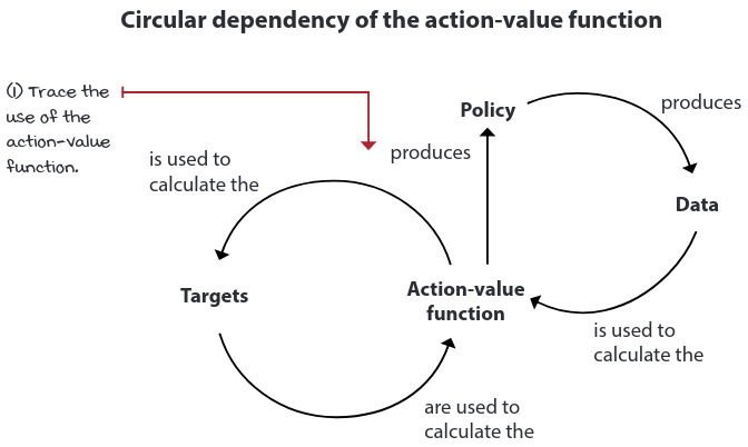
Circular dependency is actually bad, because it doesn’t respect several assumptions made in supervised learning problems.

Selecting an optimization method

Gradient descent is a stable optimization method given a couple of assumptions:

• data must be independent and identically distributed (IID)
• targets must be stationary

In reinforcement learning, however, we cannot ensure any of these assumptions hold, so choosing a robust optimization method to minimize the loss function can often make difference between convergence and divergence.

In practice, both Adam and RMSprop are sensible choises for value based DRL. RMSprop is stable and less sensitive to hyperparameters.