Balancing immediate and long-term goals
Objective of decision-making agent.
At first, we might think that the agent’s goal is to find sequence of actions that can maximize the return during an episode or its entire life depending on the task.
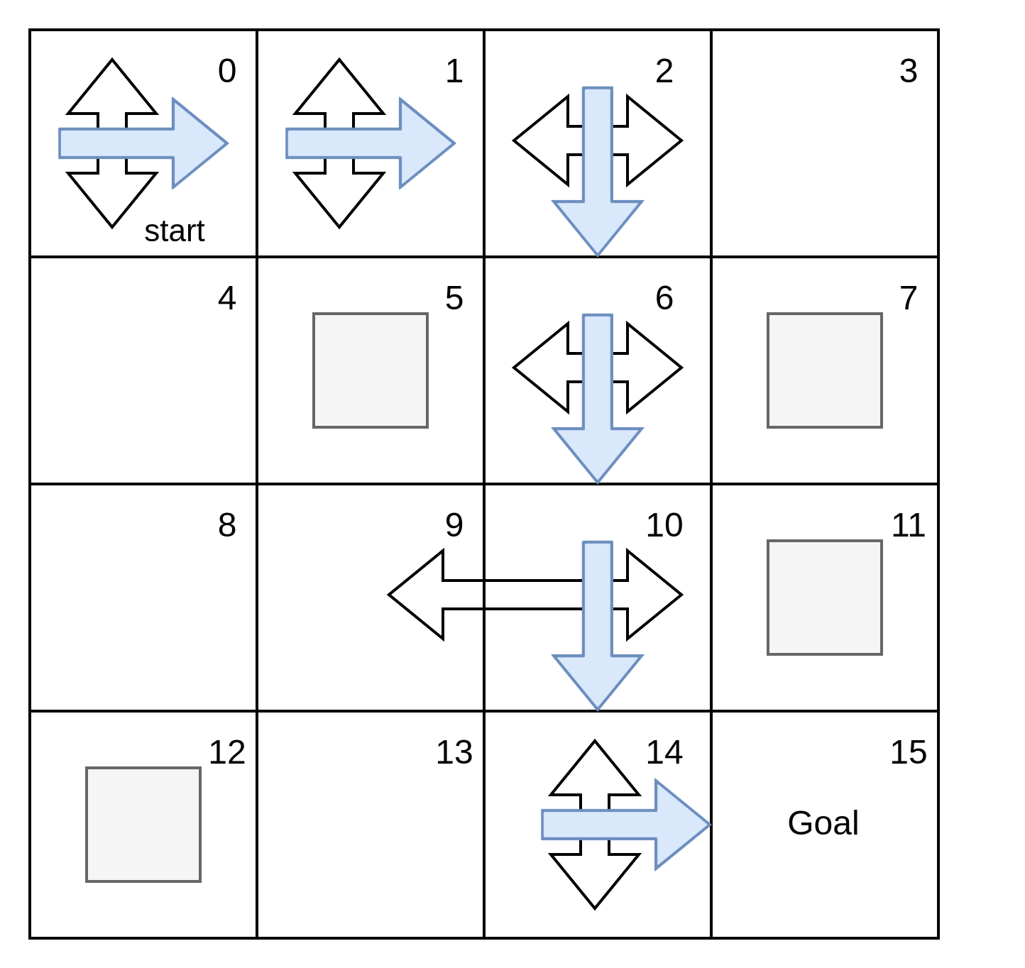
Plans are sequence of actions that agent come up with. But plans aren’t enough in a stochastic environment.
For eg.

Here, imagine that the agent is following the plan, but in state 10, the agent is sent to state 9, even if it selected the down action, as it apparenly is the right thing to do. ie. There might be a chance that unintended consequence might happen.
So we need a plan for every possible state, a universal plan, a policy.
What agent needs to come up with is called a policy. Policies are universal plans which covers all possible states. It can be stochastic or deterministic: the policy can return action-probability distributions or single actions for a given state.
Policies
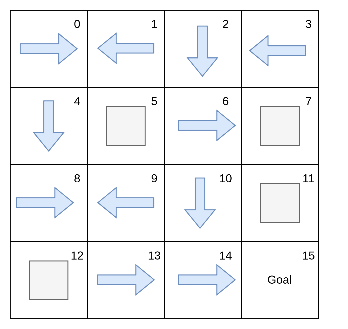
Given the stochasticity in frozen lake environment, the agent needs to find a policy, denoted as \(\pi\). A policy is a function that prescribes actions to take for a given nonterminal state. They can be stochastic.
This is a sample random policy for FL.

State-Value function
Something that would help us to compare policies is to put numbers to the state for a given policy. ie. if we’re given a policy and the MDP, we should be able to calculate the expected return starting from every single state. For instance, agent should be able to identify who much better is it to being in a state than other state? How precisely better is it? Moreover which policy have better results? and so on …
The value of state \(s\) under policy \(\pi\) is the expectation of returns if the agent follows policy \(\pi\) starting from state \(s\). Calculating this for every state, gives state-value function, or V-function or value function. It represents the expected return when following policy \(\pi\) from state \(s\).
Recursively,
\[\begin{align*} v_\pi(s) = \mathbb{E_\pi}[R_{t+1} + \gamma G_{t+1} | S_t = s] \end{align*} \\\]The next equation is called Bellman equation, which tells us how to find the value of states.
Action-value function
By comparing between different actions under the same policy, we can select better actions and therefore improve our policies. The action-value function, also known as Q-function or \(Q^\pi(s,a)\), captures precisely tge expected return if the agent follows policy \(\pi\) after taking action a in state s.
The action-value function Q,
The Bellman equation for action value is defined as follows:
\[\begin{align*} q_\pi(s,a) = \sum_{s',r}p(s', r|s,a)[r + \gamma v_\pi(s')], \forall s \in S, \forall a \in A(s) \end{align*} \\\]We don’t weight over actions because we’re interested only in a specific action.
Action-advantage function
The advantage of action a in state s under policy \(\pi\) is:
The advantage function describes how much better it is to take action a instead of following policy \(\pi\): the advantage of choosing action a over the default action.
Optimality
Policies, state-value functions, action-value functions, and action-advantage functions are the components we use to describe, evaluate and improve behaviors. We call it optimality when these components are the best the can be. An optimal policy is a policy that for every state can obtain expected returns greater than or equal to any other policy. An optimal state-value function is a state-value function with the maximum value across all policies for all states. Likewise, an optimal action-value function is an action-value function with the maximum value across all policies for all state-action pairs. The optimal action-advantage function follows a similar pattern, but notice an optimal advantage function would be equal to or less than zero for all state-action pairs, since no action could have any advantage from the optimal state-value function.
The Bellman optimality equations
The optimal state-value function:
\(\begin{align*}
v_*(s) = \underset{\pi}{max}\space v_\pi(s), \forall s \in S
\end{align*} \\\)
The optimal action-value function:
\(\begin{align*}
v_*(s) = \underset{\pi}{max}\space q_\pi(s,a), \forall s \in S, \forall a \in A(s)
\end{align*} \\\)
or, state-value function =
\[\begin{align*} v_*(s) = \underset{\pi}{max}\space \sum_{s',r}p(s',r|s,a)[r+\gamma v_*(s')] \end{align*} \\\]and action-value function =
\[\begin{align*} q_*(s,a) = \sum_{s',r}p(s',r|s,a)[r+\gamma \underset{a'}{max}\space q_*(s',a')] \end{align*} \\\]Policy evaluation
We know that policy \(\pi\) is better than or equal to policy \(\pi '\) if the expected return is better than or equal to \(\pi '\) for all states. An algorithm which we use for evaluating an arbitrary policy is known as iterative policy evaluation or just policy evaluation. The policy-evaluation algorithm consists of calculating the V-function for a given policy by sweeping through the state space and iteratively improving the estimates.
The policy-evaluation algorithm consist of iterative approximation of the state-value function of the policy under evaluation. The algorithm converges as k approaches infinity.
We have a deterministic policy, so \(\begin{align*} \sum_a \pi(a|s) = 1 \end{align*} \\\)
The policy-evaluation algorithm:
def policy_evaluation(pi, P, gamma = 1.0, theta = 1e-10):
    """
    This is a full implementation of the policy-evaluation algorithm.
    We need policy we're trying to evaluate and the MDP the policy runs on.
    """
    prev_V = np.zeros(len(P))
    while True:
        V = np.zeros(len(P))
        for s in range(len(P)):
            for prob, next_state, reward, done in P[s][pi[s]]:
                V[s] += prob * (reward + gamma * prev_V[next_state] * (not done))
        if np.max(np.abs(V - prev_V)) < theta:
            break
        prev_V = V.copy()
    return V
Policy-improvement equation
To improve a policy, we use a state-value function and an MDP to get a one-step look-ahead and determine which of the actions lead to the highest value. This is the policy-improvement algorithm.
\[\begin{align*} \pi'(s) = \underset{a}{argmax} \sum_{s'r}p(s',r|s,a) [r+\gamma v_\pi(s')] \end{align*} \\\]This is how we can implement the algorithm in python
def policy_improvement(V, P, gamma = 1.0):
    """
    It takes state-value function of policy to improve(V), MDP (P) and gamma.
    Returns the improved greedy policy by taking argmax of the Q-function of original policy.
    """
    Q = np.zeros((len(P), len(P[0])), dtype = np.float64)
    for s in range(len(P)):
        for a in range(len(P[s])):
            for prob, next_state, reward, done in P[s][a]:
                Q[s][a] += prob* (reward + gamma * V[next_state] * (not done))
    new_pi = lambda s: {s: a for s, a in enumerate(np.argmax(Q, axis =1))}[s]
    return new_pi
Policy-iteration
The plan with adversarial policy is to alternate between policy-evaluation and policy improvement until the policy coming out of the policy-improvement phase no longer yields a different policy.
def policy_iteration(P, gamma = 1.0, theta = 1e-10):
    random_actions = np.random.choice(
        tuple(P[0].keys()), len(p))
    pi = lambda s: {s:a for s,a in enumerate(random_actions)}[s]

    while True:
        old_pi = {s: pi(s) for s in range(len(P))}
        V = policy_evaluation(pi, P, gamma, theta)
        pi = policy_improvement(V, P, gamma)
        if old_pi == {s: pi(s) for s in range(len(P))}:
            break

    return V, pi
The value-iteration equation :
\(\begin{align*} v_{k+1}(s) = \underset{a}{max}\sum_{s',r}p(s',r|s,a)[r + \gamma v_k(s')] \end{align*} \\\)
The value-iteration algorithm:
def value_iteration(P, gamma = 1.0, theta = 1e-10):
    V = np.zeros(len(P), dtype = np.float64)
    while True:
        Q = np.zeros((len(P), len(P[0])), dtype=np.float64)
        for s in range(len(P)):
            for a in range(len(P[s])):
                for prob, next_state, reward, done in P[s][a]:
                    Q[s][a] += prob* (reward + gamma * V[next_state] * (not done))
        if np.max(np.abs(V - np.max(Q, axis = 1))) < theta:
            break
        V = np.max(Q, axis = 1)
    pi = lambda s: {s:a for s, a in enumerate(np.argmax(Q, axis=1))}[s]
    return V,  pi