Components of Reinforcement Learning

The two core components of RL are the agent and environment. The agent makes the decision and is generally a solution to the problem. Meanwhile the environment is the representation of problem. The agent attempts to influence the environment through actions, and the environment reacts to the agent’s actions.

The Agent: Decision maker

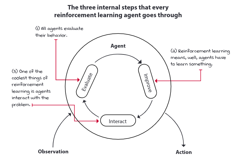
Agents are the decision makers in RL. If we zoom in, we would see that most of the agents have 3-step process; all agents have an interaction component, a way to gather data; all agents evaluate their current behavior; and all agents improve something in their inner components that allow them to improve their overall performance.

The environment

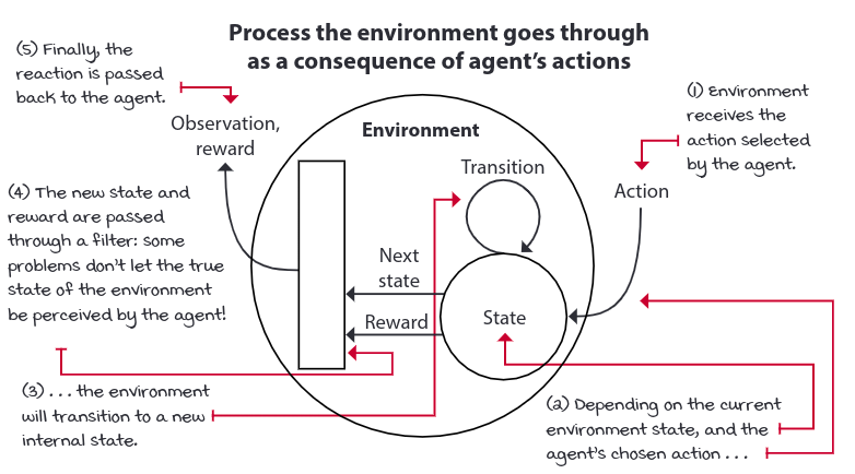
Most real-world decision-making problems can be expressed as RL environment. A common way to represent decision-making process in RL is by modeling the problem using a mathematical framework called Markov’s Decision Process(MDP).
To represent the ability to interact with an environment in an MDP, we need states, observations, actions, a transition and a reward function.

The sum of rewards we receive after single episode is called return, and Agents are often designed to maximize the return. A time step limit is often added to continuing tasks, so they become episodic tasks, and agents can maximize the return. In reality, RL agents don’t need to know the precise MDP of a problem to learn robust behaviors.

MDPs

The Frozen Lake environment

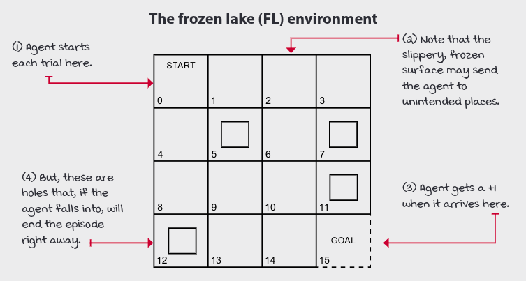
The Frozen Lake environment is a 4×4 grid which contain four possible areas  — Safe (S), Frozen (F), Hole (H) and Goal (G). The agent moves around the grid until it reaches the goal or the hole. If it falls into the hole, it has to start from the beginning and is rewarded the value 0. The process continues until it learns from every mistake and reaches the goal eventually. 

Here is visual description of the Frozen Lake grid (4×4):

Now, we will start by building a representation of MDP, using python dictionary.

States

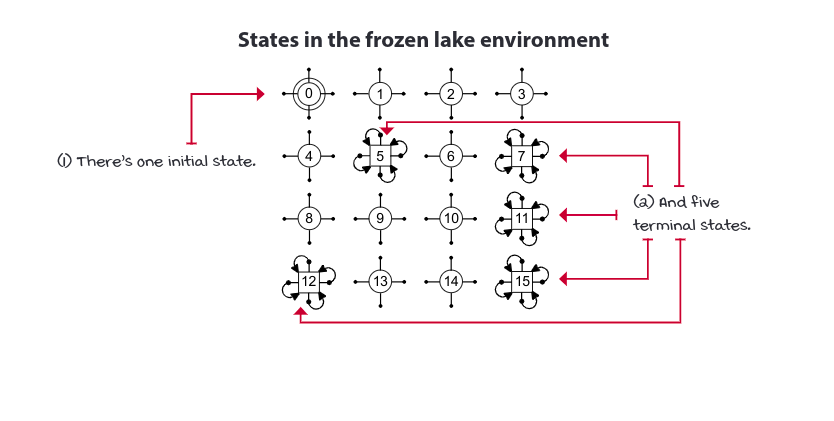
A state is a unique and self-contained configuration of the problem. The set of all possible states, the state space, is defined as the set S. The state space can be finite or infinite. In the FL, we set ids from zero to 15. In the case of MDPs the states ar fully observable; we can see the internal state of the environment at each time step, ie. observation and states are the same. Partially observable Markov decision processes (POMDPs) is a more general framework for modeling environments in which observation, which still depends on the internal state of the environment, are the only things the agent can see. State must contain all the variables necessary to make them independent of all other states.
The probability of the next state, given the current state and action, is independent of the history of interactions. This memoryless property of MDP’s is known as the Markov property: the probability of moving from one state to another on two seperate occasion, give the same action a, is the same regardless of all previous states or actions encountered before that point.

\[\begin{align*} P(S_{t+1} | S_t, A_t) = P(S_{t+1} | S_t, A_t,S_{t-1},A_{t-1},\cdots) \end{align*} \\\]

The set of all states in the MDP is denoted as \(S^+\). There is a subset of \(S^+\) called the set of starting or initial states, denoted \(S^i.\) To begin interacting with an MDP, we draw a state from \(S^i\) from a probability distribution. This distribution can be anything, but it must be fixed throughout training; ie. the probabilities must be same throughout the episode. There’s a unique state called absorbing or terminal state, and the set of all non-terminal states is denoted as \(S\). A terminal state is a special state; it must have all actions transitioning, with probability 1, to itself, and these transitions must provide no reward.

Actions: Mechanism to influence the environment

MDP’s make available a set of actions A that depends on the state. ie. There might be actions that aren’t allowed. A is actually a functions which takes current state as input. The environment makes the set of all available actions and agents can select them either deterministically or stochastically.

Transition function

The way the environment changes as response to actions is referred to state-transition probabilities or transition function, and is denoted by T(s,a,s’). The transition function T maps a transition tuple s,a,s’ to a probability; ie, passing a state s, action a and next state s’ will return the corresponding probability of transition from state s to s’ when talking an action a.
T also describes a probability distribution p(.|s, a) determining how the system will evolve in an interaction cycle from selection action a in state s.

\[\begin{align*} p(s'|s,a) = P(S_t = s'|S_{t-1}, A_{t-1} = a) \end{align*} \\\]

Also,

\[\begin{align*} \sum_{s' \in S}p(s'|s, a) = 1, \forall s \in S, \forall a \in A(s) \end{align*} \\\]

Reward signals

The reward function R maps a transition tuple s,a,s’ to a scalar. The reward can be either positive or negative. The scalar coming out of the reward function is referred to as reward. We can represent our reward function as R(s,a,s’) and also can be expressed as R(s,a) and also R(s) according to our needs. We can marginalize over next states in R(s,a,s’) to obtain R(s,a) and same for R(s,a) to R(s). But we can’t recover R(s,a) or R(s,a,s’) once we are in R(s) and cannot recover R(s,a,s’) when we are in R(s,a).

\[\begin{align*} r(s,a) = \mathbb{E}[R_t|S_{t-1} = s, A_{t-1} = a] \end{align*} \\\] \[\begin{align*} r(s,a,s') = \mathbb{E}[R_t|S_{t-1}=s, A_{t-1} = a, S_t = s'] \end{align*} \\\]

\(\begin{align*} R_t \in R \subset \mathbb{R} \end{align*} \\\) ie. Reward at time step t comes from a set of real rewards R, which is a subset of Real numbers.

Horizon

Episoidic and continuing task can be defined from the agents perspective. We call it the planning horizon. A finite horizon is a planning horizon in which the agent knows the task will terminate after an finite no of steps. An infinite horizon (indefinite horizon) is when the agent doesn’t have predetermined time step limit, so agent plans for an infinite no of time steps.
For tasks in which agent may gets stuck in a loop or mayn’t terminate, we add an artificial terminal state based on the time step.

Discount

Because of possibility of infinite sequence of time steps in indefinite horizon tasks, we need a way to discount to value of rewards over time; ie. to tell agent that getting +1s is better soon than later. We commonly use a positive real value less than one to exponentially discount the value of future rewards. This number is called discount factor or gamma. It adjust the importance of rewards over time. The later we receive rewards, the less attractive they are to present calculations.

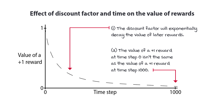
The sum of all rewards during th course of an episode is referred to as return. \(\begin{align*} G_t = R_{t+1} + R_{t+2} + \cdots + R_T \end{align*} \\\)

We can use discount factor and obtain the return. The discounted return will downweight rewards that occur later during the episode.

\[\begin{align*} G_t = R_{t+1} + \gamma R_{t+2} + \gamma^2 R_{t+3} + \cdots + \gamma^{T-1}R_T \end{align*} \\\]

or,

\[G_t = \sum_{k=0}^{\infty} \gamma^k R_{t+k+1}\]

(general form) and,

\[G_t = R_{t+1} + \gamma G_{t+1}\]

(recursive form)

There are many extensions to the MDP framework which allows us to targetslightly different types of RL problems. These are some acronyms:

• Partially Observable Markov Decision Process (POMDP) : When the agent cannot fully observe the environment state.
• Factored Markov Decision Process (FDMP): Allow the representation of the transition and reward funtion more compactly so that we can represent large MDP’s.
• Continuous [Time∣Action∣State] Markov Decision Process: When either time, action, state or any combination of them are continuous.
• Relational Markov Decision Process(RMDP):Allows the combination of probabilistic and relational knowledge.
• Semi-Markov Decision Process(SMDP): Allows the inclusion of abstract actions that can take multiple time steps to complete.
• Multi-agent Markov Decision Process(MMDP):Allow the inclusion of multiple agents in the same environment.
• Decentralized Markov Decision Process(Dec-MDP):Allows for multiple agents to collaborate and maximize a common reward.

MDPs vs. POMDPs

\[\begin{align*} MDP(S,A,T,S_\theta, \gamma, H)\end{align*} \\\] \[\begin{align*} POMDP(S,A,T,R,S_\theta, \gamma, H, O, E) \end{align*} \\\]

with, state Space \(S\), action space \(A\), transition function \(T\), reward signal \(R\). They also has a set of initial state distribution \(S_\theta\), discount factor \(\gamma\), and horizon \(H\). And for POMDP, we add the observation space \(O\) and emission probablity \(\epsilon\) that defines the probablity of showing an observation \(O\), given a state \(S\).